Accessing the whole population in most cases is not possible. Even when it’s possible, the costs of conducting a census can be astronomically high. What we do instead is take a sample and estimate statistics of interest from it.
Suppose we are interested in finding out the average salary of students who graduated recently. Since it’s very likely that the population income distribution is not normal, we take a sample of at least 30 graduates to assume approximate normality for the sampling distribution. This assumption makes inference simple, accurate, and widely applicable thanks to the Central Limit Theorem.
Our sample mean is a point estimator of our population mean. However, this estimate is almost always different from the population mean. The probability that a continuous random variable will equal a specific value is 0; that is, the probability that \bar{x} will exactly equal \mu is 0. For this reason, we use interval estimators. An interval estimator draws inferences about a population by estimating the value of an unknown parameter using an interval.
The interval is closely related to how confident we would like to be about our inference. The higher the level of confidence, the wider the interval will be. That level of confidence, which is a percentage, refers to the area under the normal distribution curve.
Let’s get back to our example to make this clearer. Suppose that after surveying 30 graduates, the salaries are as follows:
63000, 109000, 128000, 130000, 89000, 80000, 66000, 129000, 125000, 75000, 84000, 61000, 66000, 71000, 79000, 63000, 138000, 117000, 135000, 63000, 105000, 140000, 73000, 101000, 111000, 107000, 131000, 110000, 81000, 113000
The mean and standard deviation are:
grad_stu <- c(
  63000, 109000, 128000, 130000, 89000,
  80000, 66000, 129000, 125000, 75000,
  84000, 61000, 66000, 71000, 79000,
  63000, 138000, 117000, 135000, 63000,
  105000, 140000, 73000, 101000, 111000,
  107000, 131000, 110000, 81000, 113000
  )

grad_stu.mean <- mean(grad_stu)
# 98100

grad_stu.sd <- sd(grad_stu)
# 26794.69Our sample mean is an unbiased estimator of the population mean. The next step is to calculate the standard error. Standard error (SE) is the standard deviation of a sampling distribution. It tells us how much our estimate (the mean in this case) would vary from sample to sample if we repeated the study the same way. The formula is:
SE=\frac{\sigma}{\sqrt n}However, we almost never know the standard deviation of the population (\sigma). Luckily, standard deviation is the best estimator of the population standard deviation. So the formula becomes:
SE=\frac{s}{\sqrt n}Calculating SE in R:
grad_stu.se <- grad_stu.sd / sqrt(length(grad_stu))
# 4892.018Suppose we would like to be 95% confident about where our population mean falls. To find out how many standard deviations 95% is away from the mean, we can either use Student t distribution table or use R:
qt95 <- qt(.975, df = length(grad_stu) - 1)Please note that I’m using 0.975 because this is a two-tailed test and the 5% needs to be divided between both tails. For any confidence level, you should do this. This number is called Critical Value.
Now we have all the pieces to create our confidence interval. Our upper confidence limit (UCL) is the t critical value multiplied by the standard error plus the mean, and the lower confidence limit (LCL) is the same magnitude but subtracted from the mean:
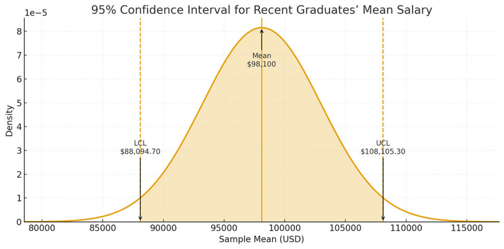
grad_stu.ci <- grad_stu.mean + c(-1, 1) * qt95 * grad_stu.se
# 88094.7 108105.3Now let’s interpret this: We are 95% confident that the population mean falls between $88,094.70 and $108,105.30. In other words, if we were to take this survey 100 times and calculate the mean, 95 of those means would fall between those two numbers.
Using Base R Function
Luckily, unless your goal is understanding the concept, there’s no need to calculate the confidence interval step by step like I did. Base R has a function that does the whole thing in one line of code:
t.test(grad_stu, conf.level = .95)

#  One Sample t-test
#
# data: grad_stu
# t = 20.053, df = 29, p-value < 2.2e-16
# alternative hypothesis: true mean is not equal to 0
# 95 percent confidence interval:
# 88094.7 108105.3
# sample estimates:
# mean of x
# 98100As you can see, R calculated the confidence interval along with some more information.
Here is the complete code:
grad_stu <- c(
  63000, 109000, 128000, 130000, 89000,
  80000, 66000, 129000, 125000, 75000,
  84000, 61000, 66000, 71000, 79000,
  63000, 138000, 117000, 135000, 63000,
  105000, 140000, 73000, 101000, 111000,
  107000, 131000, 110000, 81000, 113000
  )

grad_stu.mean <- mean(grad_stu)
grad_stu.sd <- sd(grad_stu)
grad_stu.se <- grad_stu.sd / sqrt(length(grad_stu))
qt95 <- qt(.975, df = length(grad_stu) - 1)
grad_stu.ci <- grad_stu.mean + c(-1, 1) * qt95 * grad_stu.se

sprintf(
  "We are 95%% confident that the population mean salary of
  graduates is between $%s and $%s.",
  formatC(grad_stu.ci[1], big.mark = ",", format = "f", digits = 2),
  formatC(grad_stu.ci[2], big.mark = ",", format = "f", digits = 2)
  )
2 responses to “From Sample to Population: A Quick Guide to Confidence Intervals with R”
This clarifies a lot of my confusion on the topic.
I love how you backed up every point with real examplesmade the whole topic so relatable and easy to understand. Thanks for putting in the time to create this!